mainDemo = new PeopleDynamicsFromFolder.default({
  target: document.querySelector("#main-demo"),
  props: {configDir: "/allpeople"}
});Conditional Image Generation
\[ \DeclarePairedDelimiters{\set}{\left\{}{\right\}} \DeclareMathOperator*{\argmax}{argmax} \DeclareMathOperator*{\softmax}{softmax} \]
Hopfield Networks are associative memories concerned with the storage and retrieval of data using a Lyapunov Function (“energy function”). A Hopfield Network’s memories are stored at local minima of this energy function. Given an initial data point, Hopfield Networks retrieve memories (perform “inference”) by explicitly descending the energy (following the negative gradient of the energy). This inference process is a dynamical system that is guaranteed to converge to the fixed points (“memories”)
We have built a Hopfield Network (specifically, a Dense Associative Memory) demo that runs live in your web browser. The data stored in the network are the headshots of each person responsible for putting together the AMHN Workshop @NeurIPS 2023. The animation below has two states:
- the selected person (the “label”)
- the currently displayed image (the “dynamic state”)
At every step, we display the recent history of energy values as a lineplot alongside a 2-D PCA projection of the current dynamic state (image). Watch as the dynamic state moves around the energy landscape characterized by local minima at each person!
The animation runs continously, taking small steps down the predicted energy of each (label, dynamic_state) pair. If it looks like the animation stops running when the picture is clear, it is only because we have reached the appropriate local minimum of the energy: the model is still subtracting the energy gradient from the image (it so happens that the energy gradient is zero when the dynamic state equals the original headshot).
See the description below for a more technical description.
The Anatomy of our Hopfield Network
An Associative Memory is a dynamical system that is concerned with the memorization and retrieval of data.
The structure of our data in the demo above is a collection of (image, label) pairs, where each image variable \(x \in \mathbb{R}^{3N_\text{pixels}}\) is represented as a rasterized vector of the RGB pixels and each label variable \(y \in \mathbb{R}^{N_\text{people}}\) identifies a person and is represented as a one-hot vector. Our Associative Memory additionally introduces a third, hidden variable for the memories \(z \in \mathbb{R}^{N_\text{memories}}\). These three variables are connected to each other via synapses (relationships).
In Associative Memories, each of these variables has both an internal state that evolves in time and an axonal state (an isomorphic function of the internal state that represents its conjugate variable under the Legendre Transform) that influences how the rest of the network evolves. This terminology of internal/axonal is inspired by biology, where the “internal” state is analogous to the internal current of a neuron (other neurons don’t see the inside of other neurons) and the “axonal” state is analagous to a neuron’s firing rate (we assume a neuron communicates to other neurons via its firing rate). We denote the axonal state of a variable with a hat: (i.e., variable \(x\) has axonal state \(\hat{x}\), \(y\) has axonal state \(\hat{y}\), and \(z\) has axonal state \(\hat{z}\))
Dynamic variables in Associative Memories have two states: an internal state and an axonal state.
We call the axonal state the *activations and they are uniquely defined by our choice of a scalar and convex Lagrangian function on that variable (Krotov 2021; Krotov and Hopfield 2021; Hoover et al. 2022). Specifically, in this demo we choose
\[ \begin{align*} L_x(x) &:= \frac{1}{2} \sum\limits_i x_i^2\\ L_y(y) &:= \log \sum\limits_k \exp (y_k)\\ L_z(z) &:= \frac{1}{\beta} \log \sum\limits_\mu \exp(\beta z_\mu) \end{align*} \]
These Lagrangians dictate the axonal states (activations) of each variable.
\[ \begin{align*} \hat{x} &= \nabla_{x} L_x = x\\ \hat{y} &= \nabla_{y} L_y = \softmax(y)\\ \hat{z} &= \nabla_{z} L_z = \softmax(\beta z) \end{align*} \]
The Legendre Transform of the Lagrangian defines the energy of each variable.
\[ \begin{align*} E_x &= \sum\limits_i \hat{x}_i x_i - L_x\\ E_y &= \sum\limits_k \hat{y}_k y_k - L_y\\ E_z &= \sum\limits_\mu \hat{z}_\mu z_\mu - L_z\\ \end{align*} \]
All variables in Associative Memories have a special Lagrangian function that defines the axonal state and the energy of that variable.
In the above equations, \(\beta > 0\) is an inverse temperature that controls the “spikiness” of the energy function around each memory (the spikier the energy landscape, the more memories can be stored). Each of these three variables is dynamic (evolves in time). The convexity of the Lagrangians ensures that the dynamics of our network will converge to a fixed point.
How each variable evolves is dictated by that variable’s contribution to the global energy function \(E_\theta(x,y,z)\) (parameterized by weights \(\theta\)) that is LOW when the image \(x\), the label \(y\), and the memories \(z\) are aligned (look like real data) and HIGH everywhere else (thus, our energy function places real-looking data at local energy minima). In this demo we choose an energy function that allows us to manually insert memories (the (image,label) pairs we want to show) into the weights \(\theta = \set{\theta^\text{image} \in \mathbb{R}^{N_\text{memories} \times 3N_\text{pixels}},\; \theta^\text{label} \in \mathbb{R}^{N_\text{memories} \times N_\text{people}}}\). As before, let \(\mu = \set{1,\ldots,N_\text{memories}}\), \(i = \set{1,\ldots,3N_\text{pixels}}\), and \(k = \set{1,\ldots,N_\text{people}}\). The global energy function in this demo is
\[ \begin{align} E_\theta &= E_x + E_y + E_z + \frac{1}{2} \left[ \sum\limits_\mu \hat{z}_\mu (\sum\limits_i \theta^\mathrm{image}_{\mu i} - \hat{x}_i)^2 - \sum\limits_i \hat{x}_i^2\right] - \lambda \sum\limits_{\mu} \sum\limits_k \hat{z}_\mu \theta^\mathrm{label}_{\mu k} \hat{y}_k\\ % E_\theta &= E_x + E_y + E_z + \frac{1}{2} \sum\limits_\mu \hat{z}_\mu (\sum\limits_i \theta^\mathrm{image}_{\mu i} - \hat{x}_i)^2 - \lambda \sum\limits_{\mu} \sum\limits_k \hat{z}_\mu \theta^\mathrm{label}_{\mu k} \hat{y}_k\\ &= E_x + E_y + E_z + E_{xz} + E_{yz} \end{align} \]
What’s up with \(E_{xz}\)?
The second term of \(E_{xz}\) removes \(E_x\) from the total energy ONLY because we chose to use L2 similarities rather than dot products. For pedagogical purposes, you can safely ignore the second term in \(E_{xz}\).
We introduce \(\lambda > 1\) to encourage the dynamics to align with the label.
Associative Memories can always be visualized as an undirected graph.
Every associative memory can be understood as an undirected graph where nodes represent dynamic variables and edges capture the (often learnable) alignment between dynamic variables. Notice that there are five energy terms in this global energy function: one for each node (\(E_x\), \(E_y\), \(E_z\))), and one for each edge (\(E_{xz}\) captures the alignment between memories and our image and \(E_{yz}\) captures the alignment between memories and our label). See Figure 1 for the anatomy of this network.
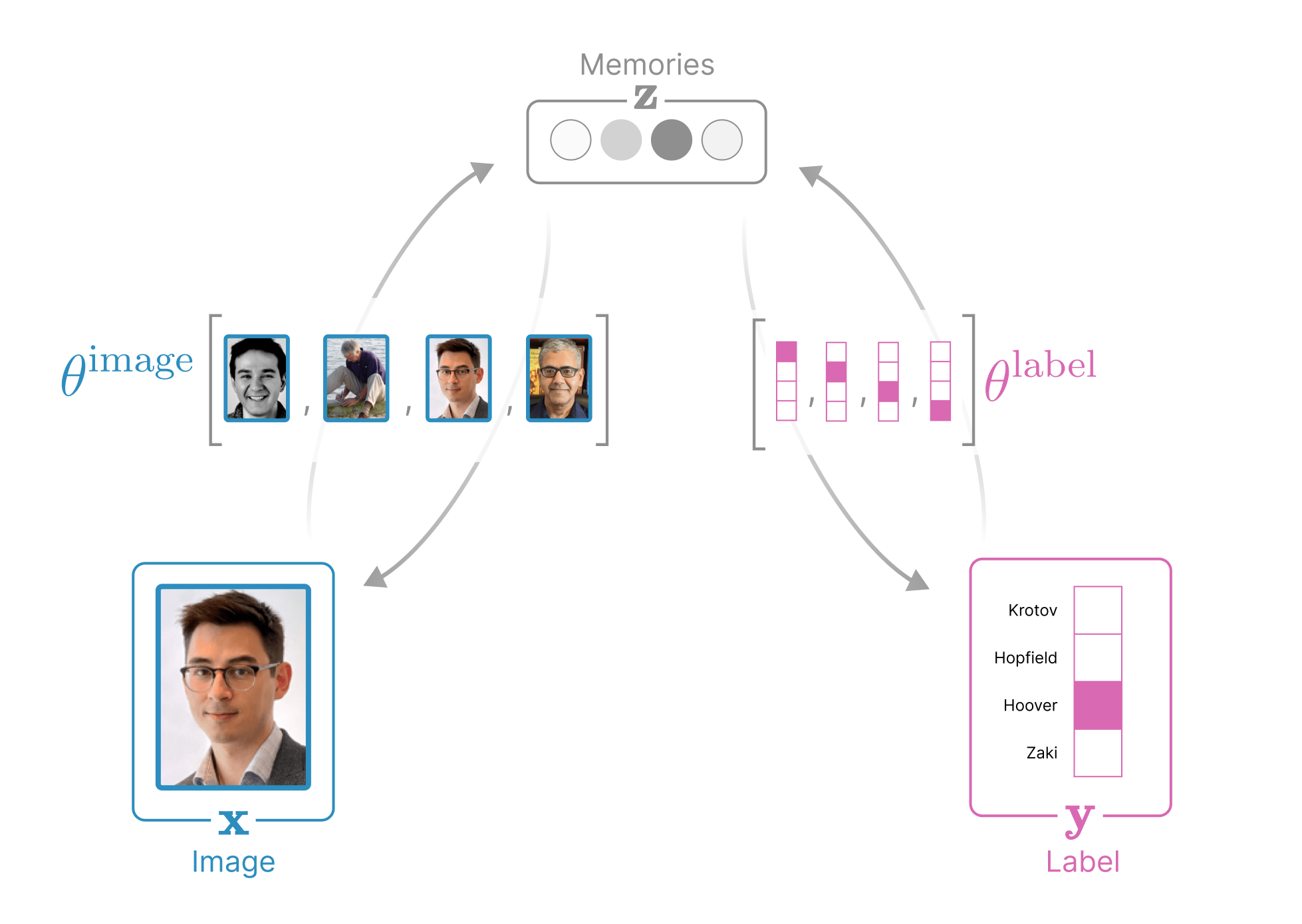
This global energy function \(E_\theta(x,y,z)\) turns our images \(x\), labels \(y\), and memories \(z\) into dynamic variables whose internal states evolve according to the following differential equations:
\[ \begin{align*} \tau_x \frac{dx_i}{dt} &= -\frac{\partial E_\theta}{\partial \hat{x}_i} = \sum\limits_\mu \hat{z}_\mu \left( \theta^\mathrm{image}_{\mu i} - \hat{x}_i \right)\\ \tau_y \frac{dy_k}{dt} &= -\frac{\partial E_\theta}{\partial \hat{y}_k} = \lambda \sum\limits_\mu \hat{z}_\mu \theta^\mathrm{label}_{\mu k} - \hat{y}_k\\ \tau_z \frac{dz_\mu}{dt} &= -\frac{\partial E_\theta}{\partial \hat{z}_\mu} = - \frac{1}{2} \sum\limits_i \left(\theta^\mathrm{image}_{\mu i} - \hat{x}_i \right)^2 + \lambda \sum\limits_k \theta^\mathrm{label}_{\mu k} \hat{y}_k - \hat{z}_\mu\\ \end{align*} \]
where \(\tau_x, \tau_y, \tau_z\) define how quickly the states evolve.
The variables in Associative Memories always seek to minimize their contribution to a global energy function.
Note that in the demo we treat our network as an image generator by clamping the labels (i.e., forcing \(\frac{d\hat{y}}{dt} = 0\)). We can similarly use the same Associative Memory as a classifier by clamping the image (forcing \(\frac{d\hat{x}}{dt} = 0\)) and allowing only the label to evolve.
The Code
The model for the above javascript demo was created using the following JAX code.
Demo Implementation, in code

Associative Memory for Face Generation
Building a simple Dense Associative Memory by inserting images into a memory matrix. Final model is converted into a TFJS binary that can be served in javascript.
!pip install einops equinox jaxtyping gdownFetch and parse data
import gdown
from pathlib import Path
force_redownload = True

ppl_id= '1oGCR84KnIwSzTfN85ikWlA4kGpYna75D'
ppl_yaml = 'workshop_people.yaml'
if force_redownload or not Path(ppl_yaml).exists():
    gdown.download(id=ppl_id, output=ppl_yaml, quiet=False)

imgs_id = '15FTnXRLBTL1oBr3GK5CbB8jfSiCZJxba'
imgs_dir = "workshop_headshots"
if force_redownload or not Path(imgs_dir).exists():
    gdown.download_folder(id=imgs_id, output=imgs_dir, quiet=False)
import yaml
import os
import numpy as np
from PIL import Image
with open(ppl_yaml, "r") as fp:
people = yaml.safe_load(fp)
headshots = [Image.open(os.path.join(imgs_dir, person["headshot"])).convert('RGB') for person in people]
assert all(h.size == headshots[0].size for h in headshots)
imgs = np.stack([np.asarray(h) for h in headshots])
img_shape = imgs.shape[1:]
img_nelements = D = imgs[0].size
Nsamples = len(imgs)
h,w,c = img_shapeCreate the Associative Memory
First, let’s import what we need to build our Associative Memory (we will use JAX – truly the best for managing complex gradient computation), and write some helper functions for converting images to vectors (to store in our Associative Memory) and back to images.
import jax
import jax.random as jr
import jax.numpy as jnp
import jax.tree_util as jtu
import equinox as eqx
import optax
from einops import rearrange
import numpy as np
from sklearn.decomposition import PCA
from PIL import Image
from jaxtyping import Float, Array

import os
from typing import *
import functools as ft
from pathlib import Path
import yaml
import json
import numpy as np

def to_imgs(x):
    """Convert weight vectors back to images"""
    x = rearrange(x, "... (h w c) -> ... h w c", h=h, w=w, c=c)
    if len(x.shape) < 4: return [Image.fromarray(np.uint8(x*255))]
    return [Image.fromarray(np.uint8(x_*255)) for x_ in x]

def to_vectors(x):
    """Convert images to weight vectors"""
    return rearrange(x, "... h w c -> ... (h w c)") / 255.
Next, let’s define our energy function using a simple Equinox module. If you paid attention to the math, you’ll notice that we took a few shortcuts in this implementation. Namely:
- We integrated out our hidden memories s.t. the whole energy function is only a function of \(x\) and \(y\) as in \(E_\theta (x, y)\).
- We assume that the labels are conditioning labels: that is, we don’t need to evolve them over time
Our Associative Memory stores \(N\) (image-label) pairs in the \(\{\theta^\text{image}, \theta^\text{label}\}\) parameters, where each image is of dimension \(D\) and each label is of dimension \(M\).
class ConditionedAssociativeMemory(eqx.Module):
    W: jax.Array
    labelW: jax.Array
    beta: float

    def __init__(self,
                 Winit:Float[Array, "N D"], # Initialize the image weights
                 labelW_init: Float[Array, "N M"], # Initialize the label weights
                 beta_init=1. # Inverse temp of the hidden units
                 ):
        self.W = jnp.array(Winit)
        self.labelW =  jnp.array(labelW_init)
        self.beta = beta_init

    def __call__(self,
                 x: Float[Array, "D"], # Dynamic image
                 labels: Float[Array, "M"], # Conditioning label
                 label_strength:float=1., # Additionally weight the label, compensates for M << D
                 ):
        """Compute the energy of the memories given a particular label"""
        assert len(x.shape) < 2, "We do not expect a batch dimension"

        sim = -jnp.sum(jnp.power(self.W - x, 2), -1)
        simlabel = label_strength * self.labelW @ labels
        energy = -jax.nn.logsumexp(self.beta * (sim + label_strength * simlabel))

        aux={}
        return energy, aux
Using the energy function…
W = to_vectors(imgs)
labels = jnp.arange(Nsamples)
labelW = jax.nn.one_hot(jnp.arange(Nsamples), num_classes=Nsamples)

label_strength=20_000 # How much more strongly to weight labels than pixels in the similarity functions
label_beta=10.
device="cpu"

# Initialize energy function
am = ConditionedAssociativeMemory(W, labelW, beta_init=10.)
Training PCAFor the demo, we will project the stored images using PCA to build intuition: for the dynamics converging to different energy minima.
# Train PCA model on the stored images
pca_model = PCA(2).fit(W)
W2 = pca_model.transform(W)
x0 = jnp.array(W[0])
To use this energy function in the frontend, we need a single function that returns the new image given the current image and a label. We also expose other things we want to show in the demo, e.g., the true energy value and the PCA projected state
def energy_and_projection_step(
        am:ConditionedAssociativeMemory, # The Associative Memory
        pcomponents, # The learned principle components of the images
        pmean, # sklearn's PCA algorithm centers the images before projecting -- this is the mean value expected
        x:Float[Array, "D"], # The dynamic image state
        label:Float[Array, "M"], # The dynamic label state
        alpha:float # The step size down the energy to take
        ):
    n_classes = am.W.shape[0]
    label = jax.nn.one_hot(label, n_classes)
    (energy, aux), grad = jax.value_and_grad(am, argnums=0, has_aux=True)(x, label, label_strength=label_strength)
    x2 = x - alpha * grad

    X = x2 - pmean
    proj_x2 = X[None] @ jnp.array(pcomponents).T
    return x2, energy, proj_x2
Quick test of the energy function:
x2, e, proj_x2 = energy_and_projection_step(am, pca_model.components_, pca_model.mean_, x0, 5, 0.05)
stepfn = ft.partial(energy_and_projection_step, am, pca_model.components_, pca_model.mean_)
Porting to ONNX
Our trained associative memory now needs to be ported to the frontend to run. For this, we will convert our model to tensorflowjs via JAX’s built-in conversion tools for tensorflow
# Don't upgrade Colab's TF version
!pip install tensorflowjs --no-deps
Requirement already satisfied: tensorflowjs in /usr/local/lib/python3.10/dist-packages (4.20.0)import tensorflow as tf
import tensorflowjs as tfjs
import tempfile
from tensorflowjs.converters import tf_saved_model_conversion_v2 as saved_model_conversion
from jax.experimental import jax2tf
from typing import *
from pathlib import Path
DType = Any
PolyShape = jax2tf.PolyShape
Array = Any
_TF_SERVING_KEY = tf.saved_model.DEFAULT_SERVING_SIGNATURE_DEF_KEY
class _ReusableSavedModelWrapper(tf.train.Checkpoint):
"""Wraps a function and its parameters for saving to a SavedModel.
Implements the interface described at
https://www.tensorflow.org/hub/reusable_saved_models.
"""
def __init__(self, tf_graph, param_vars):
"""Args:
tf_graph: a tf.function taking one argument (the inputs), which can be
be tuples/lists/dictionaries of np.ndarray or tensors. The function
may have references to the tf.Variables in `param_vars`.
param_vars: the parameters, as tuples/lists/dictionaries of tf.Variable,
to be saved as the variables of the SavedModel.
"""
super().__init__()
# Implement the interface from https://www.tensorflow.org/hub/reusable_saved_models
self.variables = tf.nest.flatten(param_vars)
self.trainable_variables = [v for v in self.variables if v.trainable]
# If you intend to prescribe regularization terms for users of the model,
# add them as @tf.functions with no inputs to this list. Else drop this.
self.regularization_losses = []
self.__call__ = tf_graph
def convert_jax(
apply_fn: Callable[..., Any],
*,
input_signatures: Sequence[Tuple[Sequence[Union[int, None]], DType]],
model_dir: str,
polymorphic_shapes: Optional[Sequence[Union[str, PolyShape]]] = None):
"""Converts a JAX function `apply_fn` to a TensorflowJS model.
Works with `functools.partial` style models if we don't need to access the variables in the frontend.
Example usage for an arbitrary function:
```
import functools as ft
import tensorflow as tf
def energy_and_projection_step(am, pcomponents, x:jnp.array, label:int, alpha:float):
...
fn = ft.partial(predict_fn, trained_model, jnp.array(pcomponents))
convert_jax(
apply_fn=fn,
input_signatures=[tf.TensorSpec((D,)), tf.TensorSpec(tuple(), dtype=tf.int32), tf.TensorSpec(tuple(), dtype=tf.float32)],
model_dir=tfjs_model_dir) # Saves model to binary files that can be loaded by tfjs
```
Note that when using dynamic shapes, an additional argument
`polymorphic_shapes` should be provided specifying values for the dynamic
("polymorphic") dimensions). See here for more details:
https://github.com/google/jax/tree/main/jax/experimental/jax2tf#shape-polymorphic-conversion
This is an adaption of the original implementation in jax2tf here:
https://github.com/google/jax/blob/main/jax/experimental/jax2tf/examples/saved_model_lib.py
Arguments:
apply_fn: A JAX function that has one or more arguments, of which the first
argument are the model parameters. This function typically is the forward
pass of the network (e.g., `Module.apply()` in Flax).
input_signatures: the input signatures for the second and remaining
arguments to `apply_fn` (the input). A signature must be a
`tensorflow.TensorSpec` instance, or a (nested) tuple/list/dictionary
thereof with a structure matching the second argument of `apply_fn`.
model_dir: Directory where the TensorflowJS model will be written to.
polymorphic_shapes: If given then it will be used as the
`polymorphic_shapes` argument for the second parameter of `apply_fn`. In
this case, a single `input_signatures` is supported, and should have
`None` in the polymorphic (dynamic) dimensions.
"""
tf_fn = jax2tf.convert(
apply_fn,
# Gradients must be included as 'PreventGradient' is not supported.
with_gradient=True,
polymorphic_shapes=polymorphic_shapes,
# Do not use TFXLA Ops because these aren't supported by TFjs, but use
# workarounds instead. More information:
# https://github.com/google/jax/tree/main/jax/experimental/jax2tf#tensorflow-xla-ops
enable_xla=False)
# Create tf.Variables for the parameters. If you want more useful variable
# names, you can use `tree.map_structure_with_path` from the `dm-tree`
# package.
# For this demo we presume that the variables are inaccessible:
param_vars = []
# param_vars = tf.nest.map_structure(
# lambda param: tf.Variable(param, trainable=False), params)
# Do not use TF's jit compilation on the function.
tf_graph = tf.function(
lambda *xs: tf_fn(*xs), autograph=False, jit_compile=False)
# This signature is needed for TensorFlow Serving use.
signatures = {
_TF_SERVING_KEY: tf_graph.get_concrete_function(*input_signatures)
}
wrapper = _ReusableSavedModelWrapper(tf_graph, param_vars)
saved_model_options = tf.saved_model.SaveOptions(
experimental_custom_gradients=True)
with tempfile.TemporaryDirectory() as saved_model_dir:
tf.saved_model.save(
wrapper,
saved_model_dir,
signatures=signatures,
options=saved_model_options)
saved_model_conversion.convert_tf_saved_model(saved_model_dir, model_dir, skip_op_check=True)Finally, let’s save our energy_and_projection_step function in an ONNX binary that can be loaded from javascript.
model_output_dir = Path("hopfield_model")
print(f"Converting to TFJS model in {model_output_dir}")

convert_jax(
    apply_fn=stepfn,
    input_signatures=[tf.TensorSpec((D,)), tf.TensorSpec(tuple(), dtype=tf.int32), tf.TensorSpec(tuple(), dtype=tf.float32)],
    model_dir=model_output_dir)

# Save model config
print(f"Caching projection of original headshots")
listW2 = W2.tolist()
for i, person in enumerate(people):
    person['proj2d'] = listW2[i]

config = {}
config['people'] = people
config['model_dir'] = str(model_output_dir)
config['img_size'] = list(img_shape)
config['Nsamples'] = Nsamples
config['nelements'] = img_nelements

print(f"Saving configuration")

with open(model_output_dir / "config.json", "w") as fp:
    json.dump(config, fp)

print(f"DONE")
Converting to TFJS model in hopfield_modelCaching projection of original headshots
Saving configuration
DONEReferences
Hoover, Benjamin, Duen Horng Chau, Hendrik Strobelt, and Dmitry Krotov. 2022. “A Universal Abstraction for Hierarchical Hopfield Networks.” In The Symbiosis of Deep Learning and Differential Equations II. https://openreview.net/forum?id=SAv3nhzNWhw.
Krotov, Dmitry, and John J. Hopfield. 2021. “Large Associative Memory Problem in Neurobiology and Machine Learning.” In International Conference on Learning Representations. https://openreview.net/forum?id=X4y_10OX-hX.